One may want to create interactive graphs by allowing users to select indicators and years to be plotted (via check boxes and scroll bars). I have presented three cases in this workbook.
↧
Control graphs with check boxes and scroll bars
↧
Extract number from an alphanumeric string
Given an alphanumeric string, one may want to perform the following
Extract phone number from the string
Assume a list of customer addresses with multiple phones numbers mentioned in the address field itself. These numbers may be mobile numbers and/or mobile numbers. Furthermore, PIN codes may also be mentioned in the address string.
One may want to extract only the phone numbers to another column.
You may refer to the my solution in this workbook.
Extract one specific 20 digit number from the string
Assume cell descriptions which contains two 20 digit numbers occurring anywhere in the string. Once may want to extract only that 20 digit number which has the word New before it.
You may refer to my solution in this workbook.
↧
↧
Extract farthest/latest date based on multiple conditions
Assume a three column database showing Site ID, Customer, Status and Requested Date. On the same site ID, the same customer may have different status on different dates. In such a scenario, one may want to know the farthest/latest requested date and its corresponding status for all unique combinations of Site ID and Customer.
I initially attempted to solve this problem by using a pivot table but the pivot output was incorrect. The pivot was returning the farthest/latest date for all status' of a particular Site ID and Customer. Ideally, it should show only the farthest/latest date and its corresponding status for a particular Site ID and Customer. Therefore, for a particular Site ID and Customer combination, only one row should show up in the final output. I ultimately solved this problem by using Advanced Filters.
You may download this workbook for a better description of the problem and my workaround.
↧
Calculate turn around time excluding Sundays and public holidays
Assume a two column database showing starting date/time and ending data/time (Data/time stamp appear in a single cell). Given a list of public holidays in a year and starting and ending work times, one may want to know the turn around time excluding Sundays and public holidays.
You may refer to my solution in this workbook.
↧
Determine the maximum number of consecutive 1′s appearing in a range
Assume a database where customers are listed from cell A6 down. From cell B5 to the right months are entered from April to March (B5:M5). In B6:M6 (Customer 1), a user enters 1's and 0's. A value of 1 respresents "Cheque bounced" and 0 represents "Cheque honoured". Similar data is entered for other customers in B7:M500.
One may want to know the maximum number of consecutive "Cheque bounce events" for all customers listed in column A without using spare rows and columns.
In cell N6, enter the following array formula (Ctrl+Shift+Enter)
=IF(MAX(FREQUENCY(IF(B6:M6=1,COLUMN(B6:M6)),IF(B6:M6=0,COLUMN(B6:M6))))=1,0,MAX(FREQUENCY(IF(B6:M6=1,COLUMN(B6:M6)),IF(B6:M6=0,COLUMN(B6:M6)))))
↧
↧
Derive end date and time from start date and time, office working hours and lunch breaks
Given the following inputs/restrictions, one may want to compute the end date and time of a project:
1. Start date and time of the project; and
2. Official working hours; and
3. Lunch breaks hours
You may refer to my solution in the this workbook.
↧
Determine cumulative expenses per employee when per diem rates vary by block of dates
Assume per diem travel rates vary by block of dates (from and to). So, assume the per diem rate for travel dates between 26/2/2013 and 28/2/2013 is Rs. 78,000/day. Likewise, if a person travels between 1/3/2013 and 25/3/2013, the per diem rate applicable is Rs. 70,000/day. With different travel dates (from and to) specified per traveller, the task is to determine total travel expenses per individual.
You may refer to my solution in this workbook.
↧
Compute MODE of all numbers split across multiple worksheets
Assume numbers are typed in range A1:A2 of multiple worksheets in a workbook. The task is the compute the MODE of these numbers. Mode is defined as the value which appears most frequently in a range of cells. So, if one types 1,3,4,3,5,6 in range A1:A6, then the mode will be 3 - 3 appears maximum number of times in the range.
In MS Excel, there is a built in way to compute the MODE. The formula for the same is
=MODE(A1:A6)
Unfortunately, MODE() is not a 3D function and therefore, something like this return a #REF error
=MODE(sheet1:sheet3!A1:A6)
This behavior seems somewhat vague because other basic Mathematical and Statistical functions such as SUM(), COUNT(), AVERAGE(), MAX(), MIN(), VAR(), and STDEV() work just fine across multiple worksheets.
To compute MODE across multiple worksheets, you may refer to my solution in this workbook.
↧
Consider a Pivot Table Value field column as a criteria for computing another Value Field column
Assume a simple three column dataset showing hours worked by different machine on different dates. So column A is Date, column B is Machine Name and column C is hours worked. There are duplicates appearing in column A and B . Blanks in column C depict machine idle time.
The task is to create a simple three column dataset showing all unique Machine names in the first column, Last day on which the machine worked in the second column and hours worked on the last day in the third column.
This problem can be solved by using formulas (Refer first worksheet of the workbook) but if one has to use a Pivot Table, then there would be a few problems.
1. The Grand Total for the Date Field should be blank because on cannot determine the Last day on which the machine worked across different machine types. A conventional Pivot Table shows the Maximum of all dates appearing in the Date Field.
2. The Grand Total for the Hours worked Field should be a summation of the total hours worked on last day across all machine types. A conventional Pivot Table shows the Maximum of all hours worked appearing in the Hours worked Field.
3. The biggest problem of them all is that there is no way to give a criteria as the Last day for that machine for computing another Field in the Pivot Table. Please refer the file for a better understanding.
This problem can be solved using the PowerPivot. You may refer to my solution in this workbook.
↧
↧
Remove special characters from a string
Hi,
Assume a column of names as follows:
Name
Mohammed Zia-Ul Haque
Steven Thomas -
,-Rohit Sunil Ahir-Chowdhary.-
Anuj -----------
Sameer --
..,Mohit --
Rajeev Nair.
Monalisa . Das
Vijeta ...
--,.Anjana. M.U..,-
Please observe that there are special characters before the name, within the name and after the name. The task is to remove special characters before and after the name. The expected result is shown below:
Expected Result
Mohammed Zia-Ul Haque
Steven Thomas
Rohit Sunil Ahir-Chowdhary
Anuj
Sameer
Mohit
Rajeev Nair
Monalisa . Das
Vijeta
Anjana. M.U
The array formula (Ctrl+Shift+Enter) to make this work is
=MID(A2,MIN(SEARCH(CHAR(ROW($A$65:$A$90)),A2&CHAR(ROW($A$65:$A$90)))),LOOKUP(2,1/((CODE(MID(UPPER(A2),ROW(INDIRECT("1:"&LEN(A2))),1))>=65)*(CODE(MID(UPPER(A2),ROW(INDIRECT("1:"&LEN(A2))),1))<=90)),ROW(INDIRECT("1:"&LEN(A2))))-(MIN(SEARCH(CHAR(ROW($A$65:$A$90)),A2&CHAR(ROW($A$65:$A$90)))))+1)
I have solved a similar problem at this link as well but that requires the usage of an add-in. This is so because the special characters and numbers need to be removed from within the string as well. In other words, everything except letters need to be removed from the alphanumeric string (no matter where the numbers and special characters are - beginning, middle or at the end).
↧
Determine number of learners who have completed different stages of multiple online courses
Here is a sample dataset of learners who have cleared different stages of multiple courses on offer within an Organisation:
| Learner | Stage completed | Course |
| Bill | Stage 1 | Public Speaking |
| Bill | Stage 2 | Public Speaking |
| Bill | Stage 3 | Public Speaking |
| Susan | Stage 1 | Effective Communication |
| Bob | Stage 1 | Public Speaking |
| Bob | Stage 2 | Public Speaking |
| Sheila | Stage 1 | Effective Communication |
| Sheila | Stage 2 | Effective Communication |
| Sheila | Stage 3 | Effective Communication |
| Frank | Stage 1 | Effective Communication |
| Frank | Stage 2 | Effective Communication |
| Henry | Stage 1 | Public Speaking |
| Henry | Stage 2 | Public Speaking |
| Bill | Stage 1 | Effective Communication |
| Bill | Stage 2 | Effective Communication |
From this sample dataset, one may want to know how many participants have completed each stage of these multiple courses. The expected result is shown below:
| Row Labels | Stage 1 | Stage 2 | Stage 3 |
| Effective Communication | 1 | 2 | 1 |
| Public Speaking | 2 | 1 | |
| Grand Total | 1 | 3 | 2 |
In this workbook, I have shared 2 solutions - one using formulas and the other using the Power Query & PowerPivot.
↧
Determine cumulative interest payable on an annuity with varying time periods
Imagine a fixed monthly amount due to an Organisation for services rendered to various customers. While an invoice is raised every month by this Organisation, not all pay up the dues on time. For unpaid dues, the Organisation charges its client interest ranging from 3% to 9% per annum. The objective is to determine cumulative interest payable by various customers to Organisation X.
The base data looks like this
| Client | Monthly revenue | Int. calculation start date | Int. calculation end date | Interest rate |
| Client A | 33,967 | 01-Aug-16 | 25-Jul-17 | 9.00% |
| Client B | 123 | 12-Sep-16 | 30-Nov-17 | 4.00% |
Given the dataset above, the total interest payable by Client A is Rs. 16,237.20. The calculation is shown below:
| From | To | Days for which interest should be paid | Principal | Interest |
| 02-Aug-16 | 31-Aug-16 | 328.00 | 33,967.00 | 2,745.26 |
| 01-Sep-16 | 30-Sep-16 | 298.00 | 33,967.00 | 2,494.17 |
| 01-Oct-16 | 31-Oct-16 | 267.00 | 33,967.00 | 2,234.71 |
| 01-Nov-16 | 30-Nov-16 | 237.00 | 33,967.00 | 1,983.62 |
| 01-Dec-16 | 31-Dec-16 | 206.00 | 33,967.00 | 1,724.16 |
| 01-Jan-17 | 31-Jan-17 | 175.00 | 33,967.00 | 1,464.70 |
| 01-Feb-17 | 28-Feb-17 | 147.00 | 33,967.00 | 1,230.34 |
| 01-Mar-17 | 31-Mar-17 | 116.00 | 33,967.00 | 970.88 |
| 01-Apr-17 | 30-Apr-17 | 86.00 | 33,967.00 | 719.79 |
| 01-May-17 | 31-May-17 | 55.00 | 33,967.00 | 460.33 |
| 01-Jun-17 | 30-Jun-17 | 25.00 | 33,967.00 | 209.24 |
| 01-Jul-17 | 25-Jul-17 | - | 33,967.00 | - |
| Total | 16,237.20 |
You may download my solution workbook with from here. I have solved this problem using normal Excel formulas and the PowerPivot.
↧
Distribute projected revenue annually
Here is a dataset showing Project wise forecast of open opportunities.
- Topic is the Project Name
- Est. Close Date is the date by when the opportunity would be closed i.e. the project would be won from that Client
- Duration is the time (in months) for which the project would run
- Amount is the total amount that would be billed for that project
Clients are invoiced annually only. So in the example below:
- Project ABC is for US$1 million with a duration of 24 months and is expected to be closed in Oct. 2017. We need to model the data to show the billing every 12 months. So for ABC US$500K would be billed in Oct-2017 and another US$500K in Oct-2018.
- Project GEF is for US$2 million with a duration of 18 months and is expected to be closed in Feb. 2018. We need to model the data to show US$1.3 million in Feb-2018 and another US$666K in Feb-2019. The monthly billing is US$2 million divided by 18 and then multiplied by 12 - this amounts to US$1.3 million.
| Topic | Est. Close Date | Duration (Months) | Amount |
| ABC | 01-10-2017 | 24 | 1,000,000 |
| GEF | 01-02-2018 | 18 | 2,000,000 |
| XYZ | 01-03-2018 | 30 | 1,000,000 |
The expected result should look like this:
| Row Labels | Oct-17 | Feb-18 | Mar-18 | Oct-18 | Feb-19 | Mar-19 | Mar-20 | Total |
| ABC | 500,000 | 500,000 | 1,000,000 | |||||
| GEF | 1,333,333 | 666,667 | 2,000,000 | |||||
| XYZ | 400,000 | 400,000 | 200,000 | 1,000,000 | ||||
| Grand Total | 500,000 | 1,333,333 | 400,000 | 500,000 | 666,667 | 400,000 | 200,000 | 4,000,000 |
I have solved this problem using Power Query and PowerPivot. You may download my solution workbook from here.
↧
↧
Determine the total number of projects by Status
Here's a simple 3 column table showing Date, Project name (Cat.) and Status of the project. Each project can have multiple status entries on different dates. So as you can observe, project "alpha_9383993" was In Progress on Oct 2, 2017, remained so on October 5, 2017 but was completed on October 6, 2017.
| Date | Cat. | Status |
| 02-Oct-17 | alpha_9383993 | In Progress |
| 03-Oct-17 | Pulse_9387388 | In Progress |
| 04-Oct-17 | Pulse_9387388 | Rework |
| 05-Oct-17 | alpha_9383993 | In Progress |
| 06-Oct-17 | alpha_9383993 | Completed |
| 07-Oct-17 | Pulse_9387388 | Completed |
| 08-Oct-17 | Oppo_tes_9383 | In Progress |
| 09-Oct-17 | Oppo_Max_8977 | Rework |
The objective is to determine the count of projects by Status as per the most recent status of every project. So the expected result is:
| Row Labels | measure 2 |
| Completed | 2 |
| In Progress | 1 |
| Rework | 1 |
The result for In Progress should be one because there is only one such project - Oppo_tes_9383. Project alpha_9383993 should not be counted because it was completed on October 6, 2017. Likewise the result for Rework should be one because there is only one such project - Oppo_Max_8977. Project Pulse_9387388 should not be counted because it was completed on October 7,2017.
I have solved this problem with the PowerPivot. You may download my solution workbook from here.
↧
Determine the most recent status after satisfying certain conditions
Assume a three column dataset with Patient ID, Smoking Status and Review Date
| PatientID | SmokingStatus | ReviewDate |
| P1 | 10-03-2018 | |
| P1 | 9 | 09-03-2018 |
| P1 | 1 | 08-03-2018 |
| P1 | 4 | 07-03-2018 |
| P2 | 9 | 10-03-2018 |
| P2 | 9 | 09-03-2018 |
| P2 | 9 | 08-03-2018 |
| P2 | 9 | 07-03-2018 |
| P3 | 2 | 10-03-2018 |
| P3 | 09-03-2018 | |
| P3 | 9 | 08-03-2018 |
| P4 | 9 | 10-03-2018 |
| P4 | 1 | 09-03-2018 |
| P4 | 4 | 08-03-2018 |
The objective is the create another 3 column dataset with the following conditions:
- If the patient's latest smoking status is other than Blank or 9, then consider that as the smoking status of the patient; and
- If the patient's latest smoking status is blank or 9, then consider the previous smoking status that is not blank or 9; and
- If the patient's smoking status is blank or 9 on all dates, then consider the smoking status as 9
The expected result is:
| PatientID | Last date when the smoking status was other than 9 or Blank | Smoking status on that date |
| P1 | 08-Mar-18 | 1 |
| P2 | 10-Mar-18 | 9 |
| P3 | 10-Mar-18 | 2 |
| P4 | 09-Mar-18 | 1 |
I have solved this question using 3 methods - PowerPivot, Advanced Filters and formulas. You may download my solution workbook from here.
↧
Filtering on 2 date fields within one Table
This table contains a list of all the inspections created and completed within different time periods.
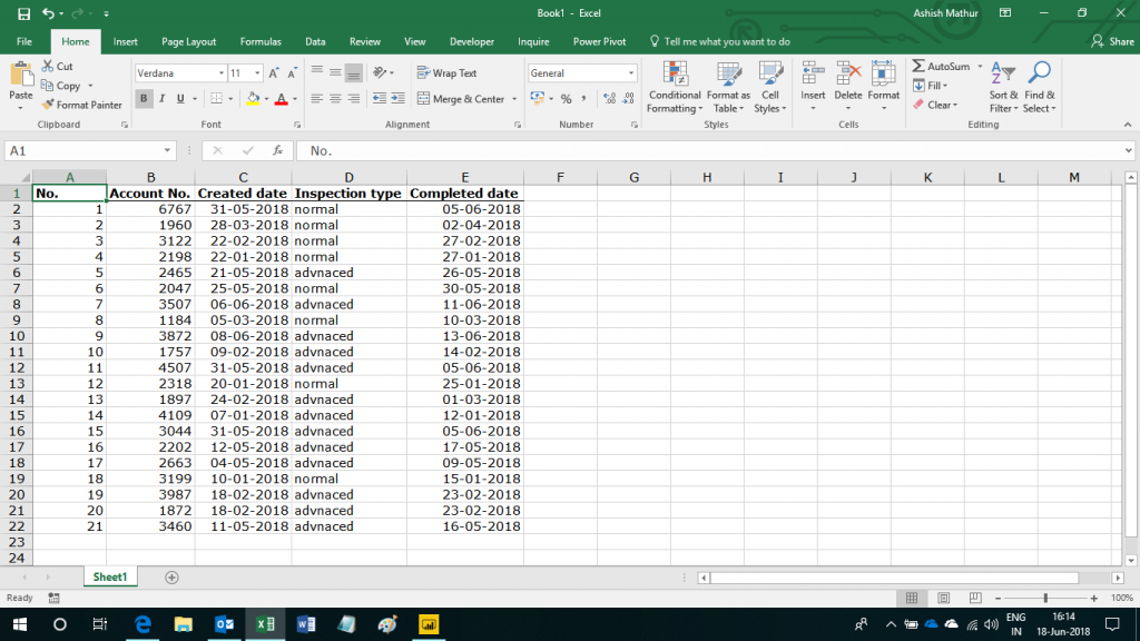
The objective is to create two Tables from this single table - one showing the Accounts created within the chosen time period and another showing the those that were closed within the same time period. Here are screenshots of the expected results.

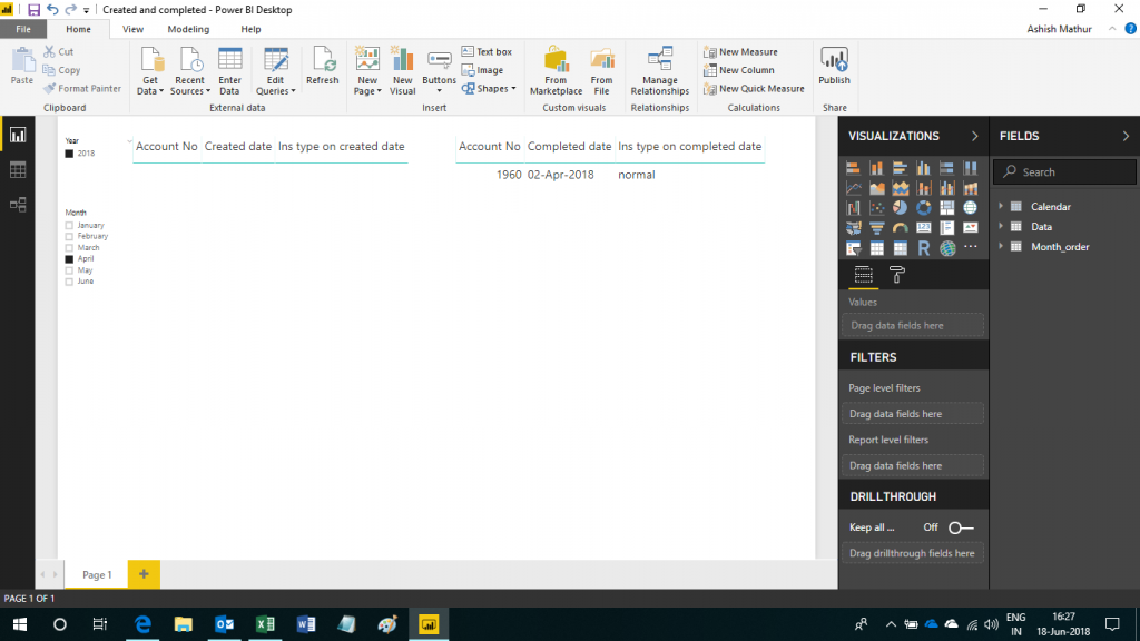
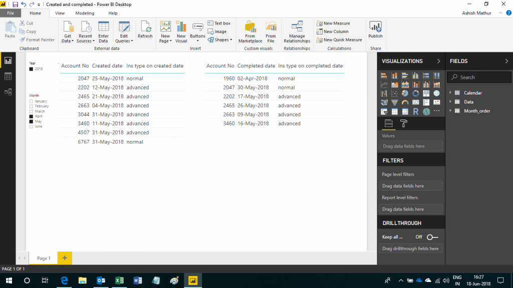
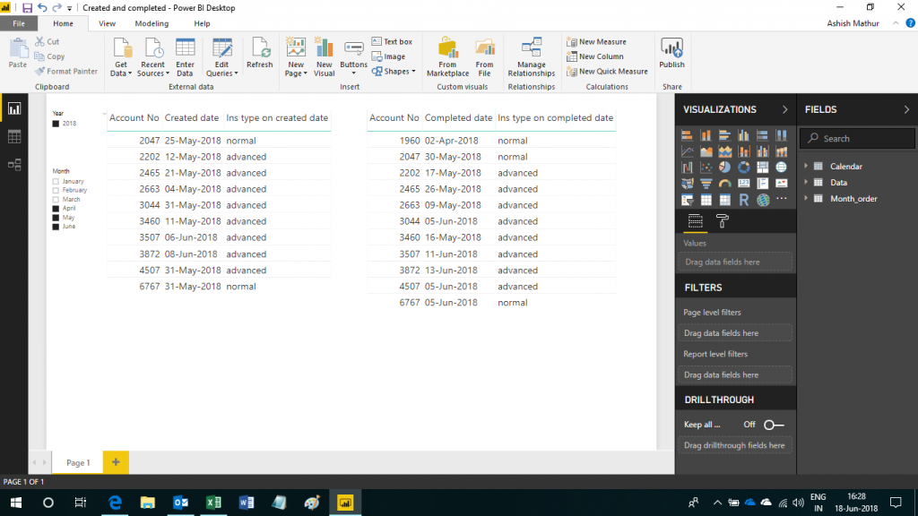
You may download my PowerBI desktop solution workbook from here. The same solution can be obtained in Excel as well (using Power Query and PowerPivot).
↧
Show sales only for corresponding months in prior years
Refer to this simple Sales dataset
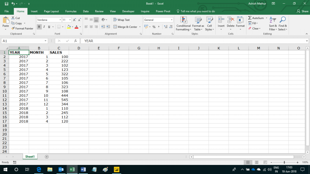
The objective is to create a simple matrix with months in the row labels, years in the column labels and sales figures in the value area section. The twist in the question is that for years prior to the current year (2018 in this dataset), sales should only appear till the month for which there is data for the current year. For e.g., for 2018, data is only till Month 4 and therefore for prior years as well, data should only appear till Month 4. As and when Sales data gets added below row 17, data for prior years should also go up to that month.
The expected result is
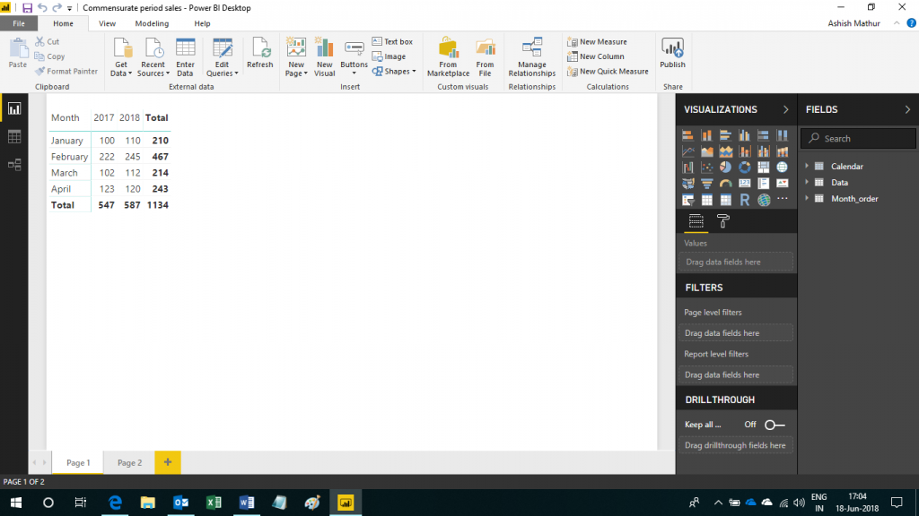
You may download my PBI file from here. The same solution can be obtained in Excel as well (using Power Query and PowerPivot).
↧
↧
Show Project wise status in a Pivot Table
Visualise a simple 6 column Table as shown below - Project Name and the finish date for each of the 5 stages that the projects go through. Each project goes through 5 stages - Requirement (Req), Development (Dev), UAT, Implement and Warranty.
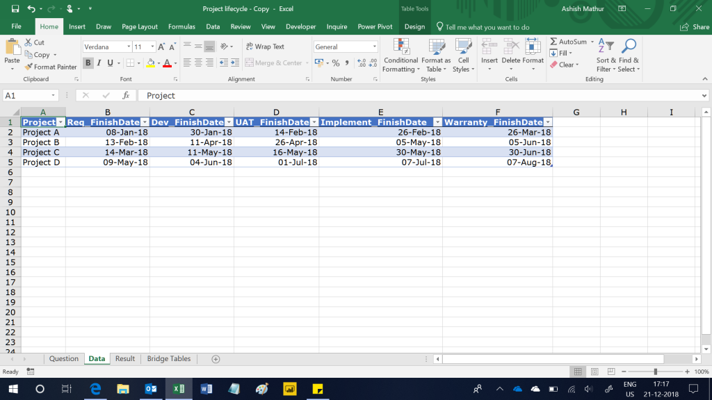
The objective is to report on the status of each project at the end of each month based on which stage is/was completed in that month. So, if a given project's requirements are completed in January and development completes some time in March, the one would expect the output of the report to show the project's status in January and February as "Req" and in March as "Dev" respectively. February should also show "Req" because the next stage was completed only in March (although it may have started in January). If multiple stages complete in one month, then the report should display only the most recently completed stage. So, if Project A completed both Requirements and Development stages in January, the report should show only "Dev" as the stage completed in January.
For the data shared above, the expected result is:
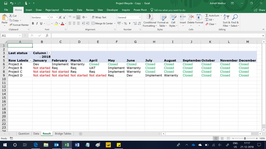
You may download my solution workbook from here.
↧
Flex a Pivot Table to show data for x months ended a certain user defined month
In this simple 3 column dataset shown below, one can see the month wise demand and energy charge for 2 years - 2017 and 2018.

The objective is to compute the month wise demand charge for x months ended a certain user defined Year and Month. So, if a user selects the Year as 2018, Month as June and Duration as 9, then the Pivot Table should show month wise demand charge for the 9 months ended June 2018 i.e. from October 2017 to June 2018. Likewise, if a user selects Year as 2018, Month as May and Duration as 3, then the Pivot Table show should month wise demand charge for the 3 months ended May 2018 i.e. March 2018 to May 2018.

You may download my solution workbook from here.
↧
Determine the top selling location for each product
Visualise a 3 column dataset as shown below - Location, Product and Sales. Each location can have multiple products (Product A has Banana, Apple and Carrot) and each product can be sold in multiple locations (Banana is sold in locations A, B and F).

The objective is to determine the location with highest sales for each product. So for Banana, maximum sale value is 25 and location of maximum sales value is B. Likewise for Orange, maximum sales value is 49 and location of maximum sales value is A. The expected result is:

I have 4 solutions to this problem:
- Advanced Filters - This is a static solution. For any changes in the source data range, one will have to re-enter the 3 inputs in the Advanced Filter window
- Formulas - This is a semi-dynamic solution. To make it fully dynamic, one will have to write an array formula to first extract all unique product names in a column. The array formula to extract product names in a column can be obtained from here.
- Power Query - This is a dynamic solution. For any changes in the source data sheet, one just has to go to Data > Refresh All
- PowerPivot - This is a dynamic solution. For any changes in the source data sheet, one just has to go to Data > Refresh All
You may download my solution workbook from here.
↧